This is why you should consider using model-based clustering
Let’s suppose you have the following data. It contains 177 wines with some characteristics about them. You’d like to group them in such way you can create a marketing campaign, for example.
set.seed(143)
pkgs <- c("mclust", "dplyr")
invisible(lapply(pkgs, require, character.only = TRUE))

df <- read.csv('https://archive.ics.uci.edu/ml/machine-learning-databases/wine/wine.data')
names(df) <- c('Type', 'Alcohol', 'Malic_acid', 'Ash', 'Alcalinity',
               'Magnesium', 'Total_phenols', 'Flavanoids',
               'Nonflavanoid_phenols', 'Proanthocyanins',
               'Color_intensity', 'Hue', 'OD280', 'Proline')
df <- df %>% select(-Type)

glimpse(df)
## Observations: 177
## Variables: 13
## $ Alcohol <dbl> 13.20, 13.16, 14.37, 13.24, 14.20, 14.39, 1…
## $ Malic_acid <dbl> 1.78, 2.36, 1.95, 2.59, 1.76, 1.87, 2.15, 1…
## $ Ash <dbl> 2.14, 2.67, 2.50, 2.87, 2.45, 2.45, 2.61, 2…
## $ Alcalinity <dbl> 11.2, 18.6, 16.8, 21.0, 15.2, 14.6, 17.6, 1…
## $ Magnesium <int> 100, 101, 113, 118, 112, 96, 121, 97, 98, 1…
## $ Total_phenols <dbl> 2.65, 2.80, 3.85, 2.80, 3.27, 2.50, 2.60, 2…
## $ Flavanoids <dbl> 2.76, 3.24, 3.49, 2.69, 3.39, 2.52, 2.51, 2…
## $ Nonflavanoid_phenols <dbl> 0.26, 0.30, 0.24, 0.39, 0.34, 0.30, 0.31, 0…
## $ Proanthocyanins <dbl> 1.28, 2.81, 2.18, 1.82, 1.97, 1.98, 1.25, 1…
## $ Color_intensity <dbl> 4.38, 5.68, 7.80, 4.32, 6.75, 5.25, 5.05, 5…
## $ Hue <dbl> 1.05, 1.03, 0.86, 1.04, 1.05, 1.02, 1.06, 1…
## $ OD280 <dbl> 3.40, 3.17, 3.45, 2.93, 2.85, 3.58, 3.58, 2…
## $ Proline <int> 1050, 1185, 1480, 735, 1450, 1290, 1295, 10…You decided in some analytical way that the number of groups that best fits your needs is 3. Then you’re probably tempted to run a K-means clustering method to build the groups. This of course makes sense, but you could get a more exciting result. Model-based clustering attempts to manage the fact that traditional clustering algorithms (like K-Means) derive their results without considering uncertainty to the cluster assignments. The most well-known approaches are probably based on Gaussian Mixture Models.
If you run the K-Means method you’ll get something like this:
km <- kmeans(df, centers = 3, iter.max = 10)

plot(df[,c(1:5)], col = c('red3', 'dodgerblue2', 'green3')[km$cluster], pch = 20, main = 'K-Means')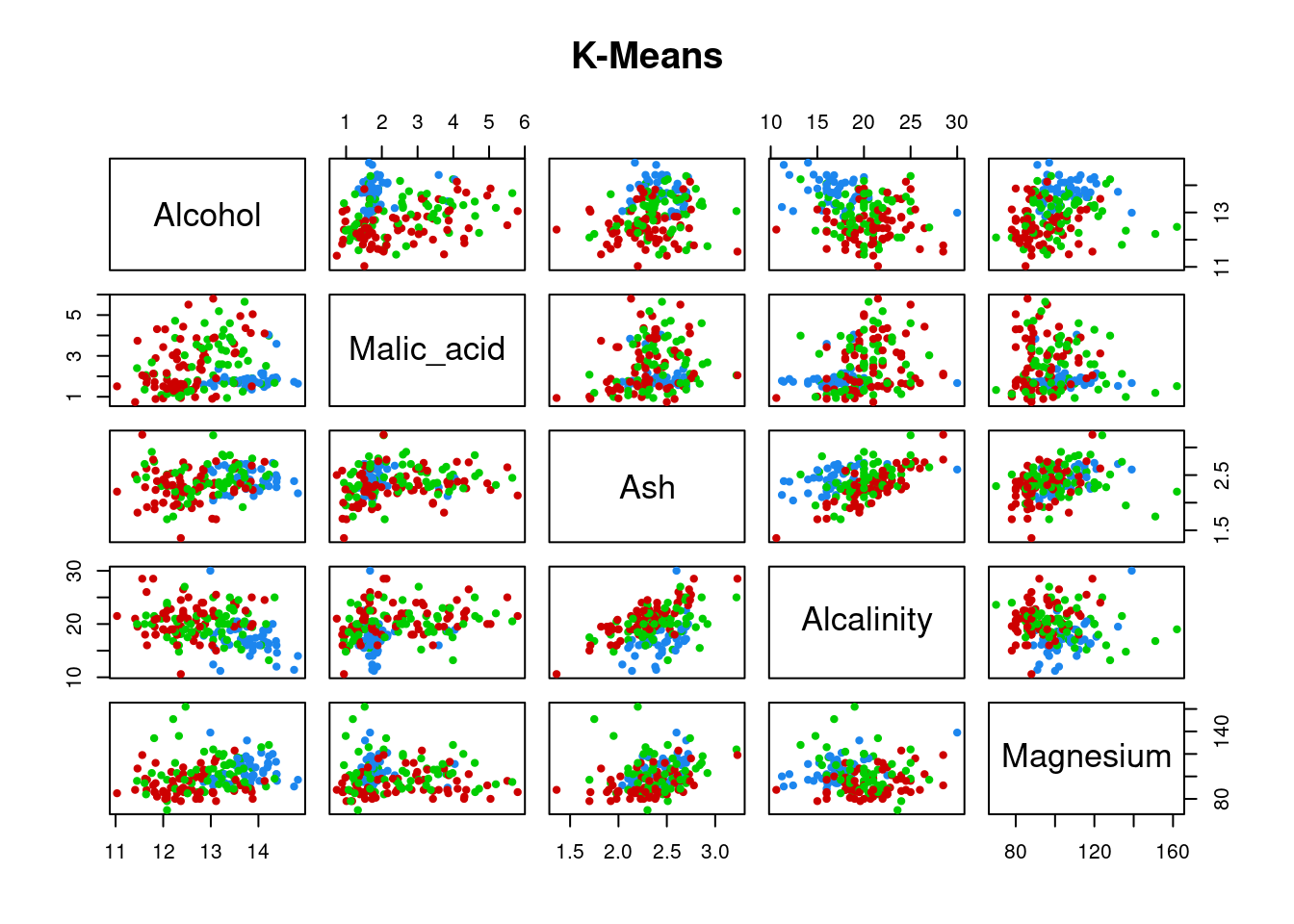
And with a Gaussian Mixture Model you could get something like:
clust <- Mclust(df, G = 3)

plot(clust, what = "uncertainty", addEllipses = FALSE, dimens = c(1:5), cex = 1.7)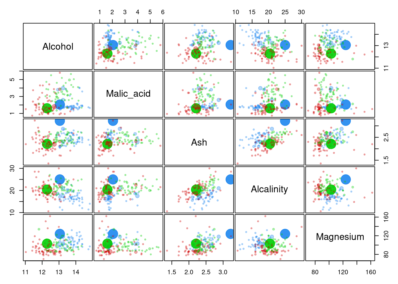
These would be the wines with the most uncertainty. Each column represents the probability that each observation belongs to that specific group.
as.data.frame(round(predict(clust, df)$z, 2))[sort(clust$uncertainty, index.return=TRUE, decreasing=TRUE)$ix[1:5],]## 1 2 3
## 70 0.00 0.22 0.78
## 25 0.78 0.22 0.00
## 81 0.03 0.97 0.00
## 43 0.98 0.02 0.00
## 4 0.99 0.01 0.00Where the larger the data point, the higher the uncertainty. In this example you might see there’re only few data points where this uncertainty is present, so it seems all clusters are well-defined, but in more complex examples this could be crucial in order to make a decision. Suppose you’d like to send emails for a specific marketing campaign. The decision of whether or not to impact customers could be relevant, so you might consider not affecting those customers who are between two groups.