Maximum Likelihood Estimation and the Newton-Raphson method
The Maximum Likelihood Estimation (MLE) is probably one of the most well-known methods for estimating the parameters of a particular statistical model, given the data. It aims at finding the parameter values that makes the observed data most likely under the assumed statistical model.
Let \(X_1, ... X_n\) be independent and identically distributed random variables. We assume that the data are drawn from a distribution with density \(f(x|\theta)\). Given the data, we define the likelihood as follows:
Then the goal of MLE is to find the parameters values that maximize the likelihood function, given the data.
I won’t go into the details but it’s quite common to take logarithms on the likelihood function (since the logarithm is a monotonically increasing function) so the maximization of the log-likelihood is equivalent to maximize the likelihood function itself and it ends up being easier to compute because the product becomes a sum.
Newton-Rapshon method
Some methods have been developed to cope with the solution when the analytical solution is hard to compute, which is true most of the times. One of them is the Newton-Rapshon algorithm, developed by Isaac Newton and Joseph Raphson, which is used to approximate roots of real-valued functions.
We start with a initial values, \(x_0\). Then, if the function satisfies the proper assumptions,
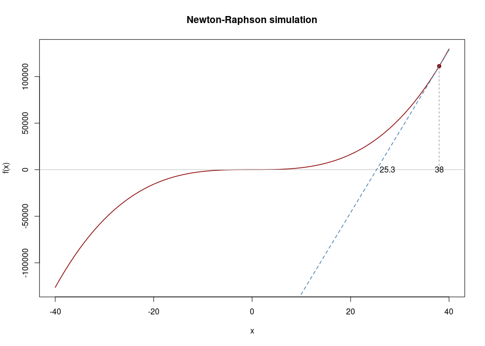
is a better approximation of the root than \(x_0\). \((x_1, 0)\) is the intersection of the x-axis and the tangent of the function at \((x_0, f(x_0))\). In the following plot our first guess \((x_0)\) is 38 and after drawing the tangent line we see that the intersection with the x-axis is at 25.3, which becomes the \(x_1\) value.
The process will be repeated as
until the difference between \(x_{n+1}\) and \(x_n\) is smaller than a tiny value (it’s called epsilon in this post).
Let’s see an example with a random function and then let’s see the application for the MLE case. Suppose we have this function (this is the function plotted above):
We also know that:
Let’s jump to the code. Define the function and its derivative:
# Function
func <- function(x) 2 * x^3 + x^2 + 10

# Derivative function
dfunc <- function(x) 6 * x^2 + 2*x
Let’s see how the code for the Newton-Raphsonm method looks like and run it:
newton_raphson <-
  function(xn, epsilon = 1e-6, n = 500) {

    # store all values
    values <- xn

    # loop n times (in this example we'll never reach the max number of iterations)
    for (i in seq_len(n)) {

      # NR equation
      xn1 <- xn - func(xn)/dfunc(xn)
      cat("Iteration", i, "Value", xn1, "\n")

      # accumulative iteration values
      values <- c(values, xn1)

      # if difference between xn1 and xn is less than epsilon, convergence reached
      if(abs(xn1 - xn) < epsilon) {
        cat("Convergence reached!", "\n")
        res <- list(final_value = values[length(values)],
                    values = values)
        return(res)
      }

      # new iteration
      xn <- xn1
    }
  }


tst <- newton_raphson(xn = 38)
## Iteration 1 Value 25.27712
## Iteration 2 Value 16.794
## Iteration 3 Value 11.13573
## Iteration 4 Value 7.356832
## Iteration 5 Value 4.821948
## Iteration 6 Value 3.095622
## Iteration 7 Value 1.856579
## Iteration 8 Value 0.7806913
## Iteration 9 Value -1.434821
## Iteration 10 Value -2.083476
## Iteration 11 Value -1.912195
## Iteration 12 Value -1.894124
## Iteration 13 Value -1.893932
## Iteration 14 Value -1.893932
## Convergence reached!This is the final value and all the previous ones, \(x_0,...,x_{15}\):
tst## $final_value
## [1] -1.893932
##
## $values
## [1] 38.0000000 25.2771167 16.7940041 11.1357341 7.3568321 4.8219479
## [7] 3.0956224 1.8565792 0.7806913 -1.4348208 -2.0834756 -1.9121949
## [13] -1.8941237 -1.8939316 -1.8939315And this would be the whole iterations process:
Poisson example
What about a “real life example”? Assume a Poisson distribution with probability mass function:
For \(X_1,...,X_n\) identically distributed random variables we have a likelihood function like:
Taking logs and reordering:
Now we find the maximum likelihood estimation by taking the derivative and equaling it to zero. This lead us to conclude that the MLE is equal to the mean:
Going back to the code, let’s now simulate 100 observations from a Poisson distribution with \(\lambda = 4\):
set.seed(123)

# Simulate 100 random values
df <- rpois(n = 100, lambda = 4)

# Mean?
mean(df)
## [1] 4.09# Probability mass function for the Poisson process
func <- function(x) {
sum(df)/x - 100
}
# Derivative from the previous function
dfunc <- function(x) {
-sum(df)/x^2
}Now, I’m going to run the Newton-Raphson method choosing \(\lambda = 7\) as starting value:
tst <- newton_raphson(xn = 7)## Iteration 1 Value 2.01956
## Iteration 2 Value 3.041902
## Iteration 3 Value 3.821416
## Iteration 4 Value 4.072362
## Iteration 5 Value 4.089924
## Iteration 6 Value 4.09
## Iteration 7 Value 4.09
## Convergence reached!
Great, the mean value is reached!
Unfortunately, as usual, there’s no free lunch. What if we had chosen a bad starting point? Well, the algorithm fail to converge and crash.
tst <- newton_raphson(xn = 15)## Iteration 1 Value -25.01222
## Iteration 2 Value -202.9857
## Iteration 3 Value -10480.1
## Iteration 4 Value -26874867
## Iteration 5 Value -1.765914e+14
## Iteration 6 Value -7.624575e+27
## Iteration 7 Value -1.421373e+55
## Iteration 8 Value -4.939609e+109
## Iteration 9 Value -5.965707e+218
## Iteration 10 Value -Inf
## Iteration 11 Value -Inf## Error in if (abs(xn1 - xn) < epsilon) {: valor ausente donde TRUE/FALSE es necesarioI’ve seen there are some mathematical approaches to deal with this, but maybe in the next chapter!