Building a simple football player rating model
This model is somehow inspired by the PlayeRank methodology developed by Pappalardo et al. (2019). You can see the work-in-progress code of the following analysis here.
This post aims to show a simple two-step model for rating football players. To this end, I’ll take the FA Women’s Super League as an example. The data comes from the StatsBomb Open Data repository, which has all the details of the events they collect.
What do I mean by rating football players? This seems a confusing term but in the end this boils down to having an objective value of the players’ performance. It’s “objective” because it’s not subject to personal views about the players at all (though, of course, the model may be biased). This performance rate ranges from 0 to 100 —meaning 0 poor performance— and it’s computed in a two-steps model. We have available the information of each event for each game, so the first step would be to have an idea on how important these events are in order to predict the match outcome. Therefore, those players who succeed in the most predominant events will have higher rating values. Thus, we have the two-steps model: the first step is to obtain the events importance and the second one is to build the rating itself throughout the weights we got in step 1.
1. Getting feature importance
We have a lot of information about the players’ perfomance in a specific match, but we should know how important a complete pass or a tackle is. For this purpose, I’ll transform the original data (at event level) in order to have something like this:
| match_id | home_score | away_score | team_type | result | complete_passes | incomplete_passes | other_variables |
|---|---|---|---|---|---|---|---|
| 19714 | 0 | 1 | home_team | 0 | 382 | 150 | … |
| 19714 | 0 | 1 | away_team | 1 | 420 | 201 | … |
| 19715 | 3 | 1 | home_team | 1 | 560 | 198 | … |
| 19715 | 3 | 1 | away_team | 0 | 364 | 269 | … |
| 19716 | 0 | 0 | home_team | 0 | 459 | 256 | … |
| 19716 | 0 | 0 | away_team | 0 | 474 | 321 | … |
For each match, I’ll have two records, one for each team. Then, the target (result column) is defined by the match outcome so it’s set to 1 in case of win and 0 in case of defeat or draw. This is of course a simplification in order to deal with a binary outcome and it works reasonably well. For the whole dataset there’re 923 defeats or draws and 675 wins. To train this model, I’ll use all the competitions and matches available in the StatsBombs repository, though I’ll only compute the FA Women’s League’s rating values afterwards, as I said.
I’ll try with three different models: a Logistic Regression, a Support Vector Machine with Linear Kernel and a Support Vector Machine with Radial Basis Kernel. These are the results after tuning some hyperparameter values of the SVM models (using a 10-fold cross-validation):
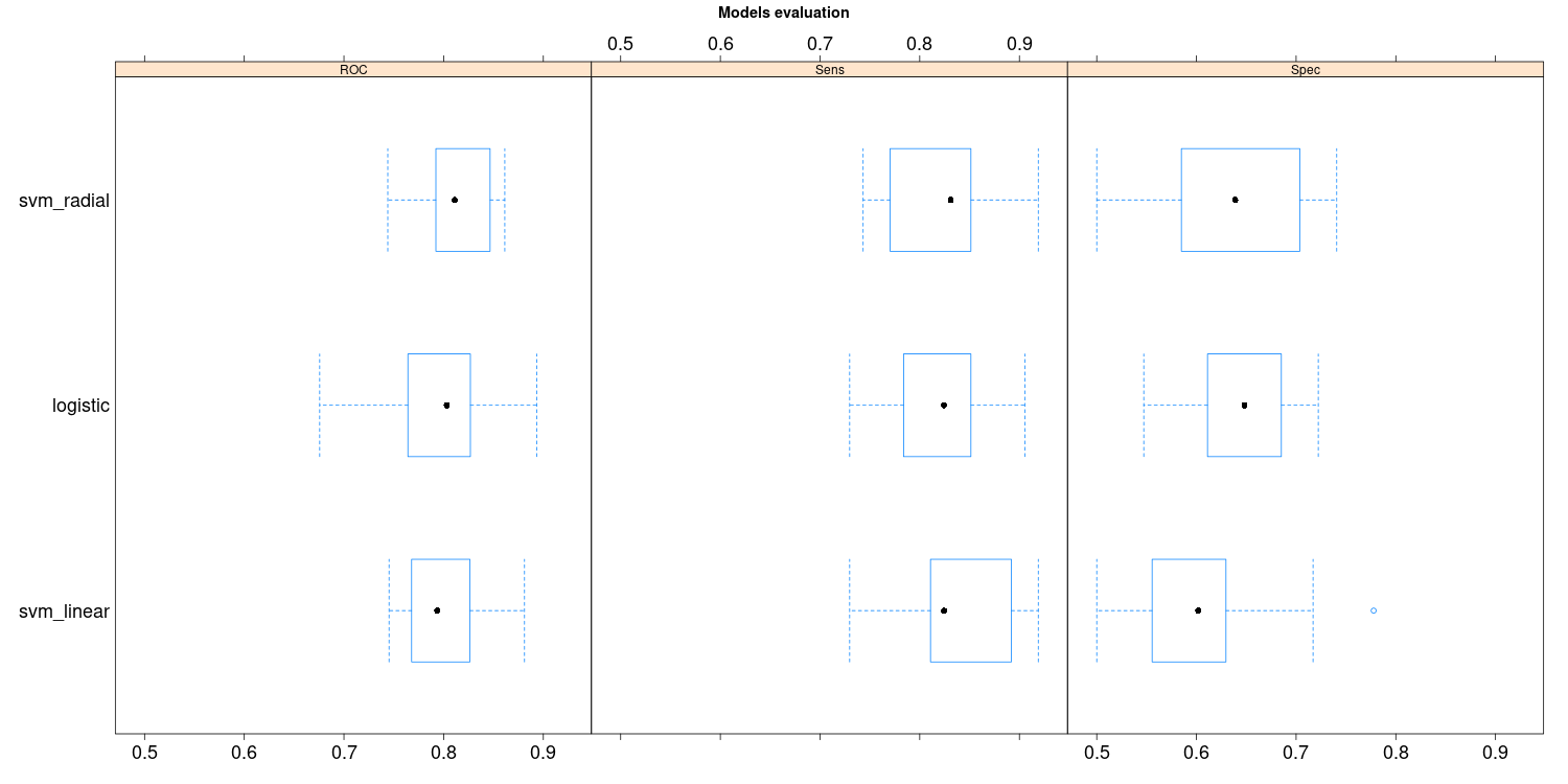
According to the results, I’ll select the SVM with Radial Kernel as the final model since it’s the one with the highest AUC value, though it’d be desirable to compare the significance of the AUCs’ differences through, for example, a permutation test.
Now, let’s see what the coefficients look like. Overall, it seems to be pretty consistent with what one might expect though there’re some variables which have the opposite sign I’d expect (like red_card) but I think this is an ocurrence issue, red cards aren’t a common events during a game and I suspect they almost always occur at the end of the matches, so this may not affect the outcome of the matches as one might expect. This is definitely something that needs to be looked at more closely. The other variable that caught my attention is goalkeeper_saves. At first glance, I thought this should have a positive impact on wins, but after further thought I realised that the more the goalkeeper is saving, the more offensive action the opponent is taking (and therefore the greater its chances of winning).
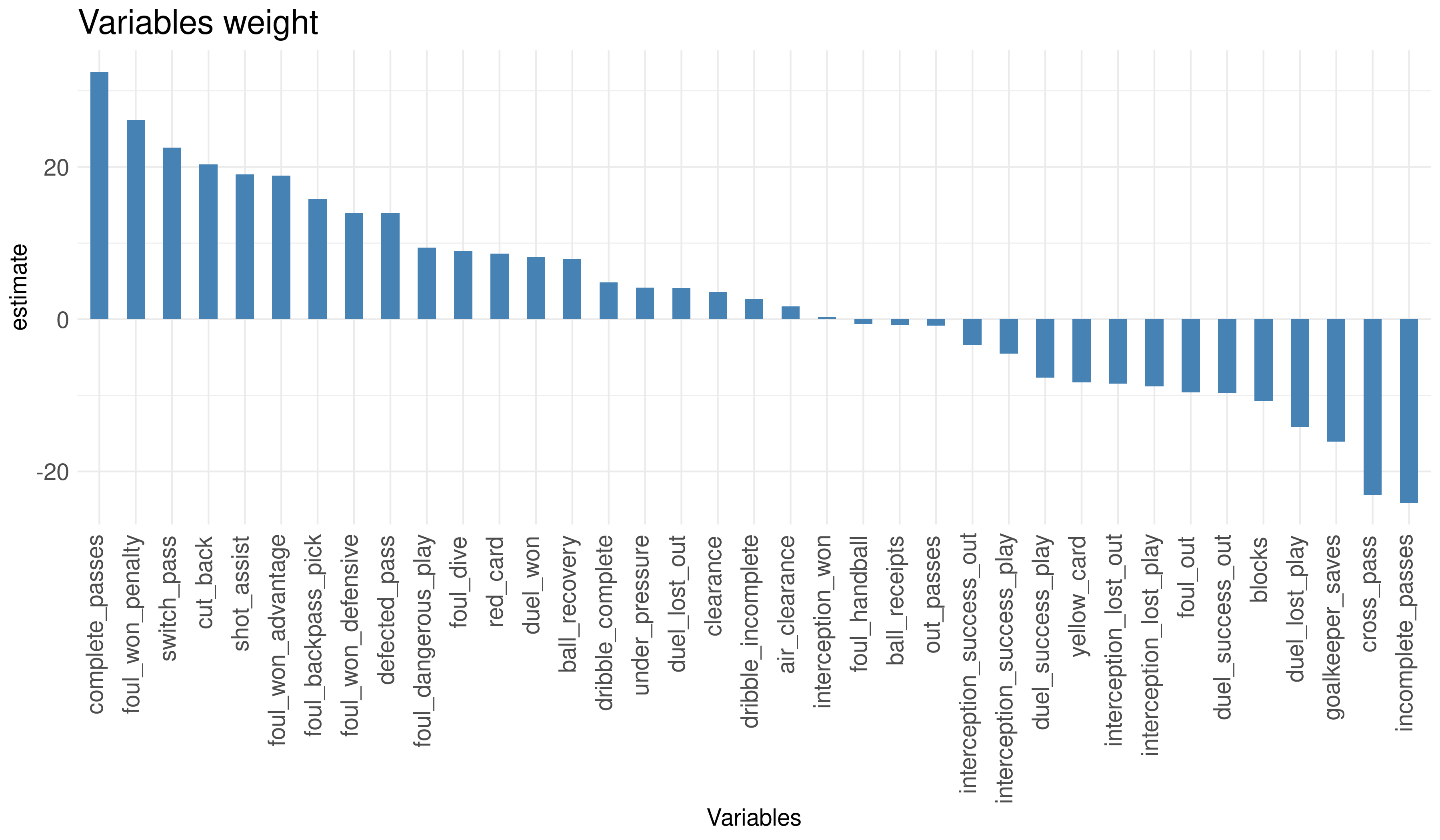
The resulting coefficients are the weights I’ll use for the second step.
2. Player Rating
In this second phase, I’ll use the coefficients to build the rating metric, which I’ll denote by \(r_i\) where \(i = \{player_1, player_2,..., player_n\}\). Now the goal is to build the same dataset as before but at player and match level. This will allow us to have the same variables with which we built the previous model. Once I have the dataset, I proceed as follows:
- I multiply each feature by its weight —coefficients of the SVM model— at game and player level.
- I add up all these weighted variables obtaining a value in the range \([0, \infty)\). Take into account that resulting values are already weighted by the minutes the players have played in that specific game!
- Then I normalize and multiply them by 100, so they’re bounded in the range \([0, 100]\).
- Finally, I compute the mean for each player.
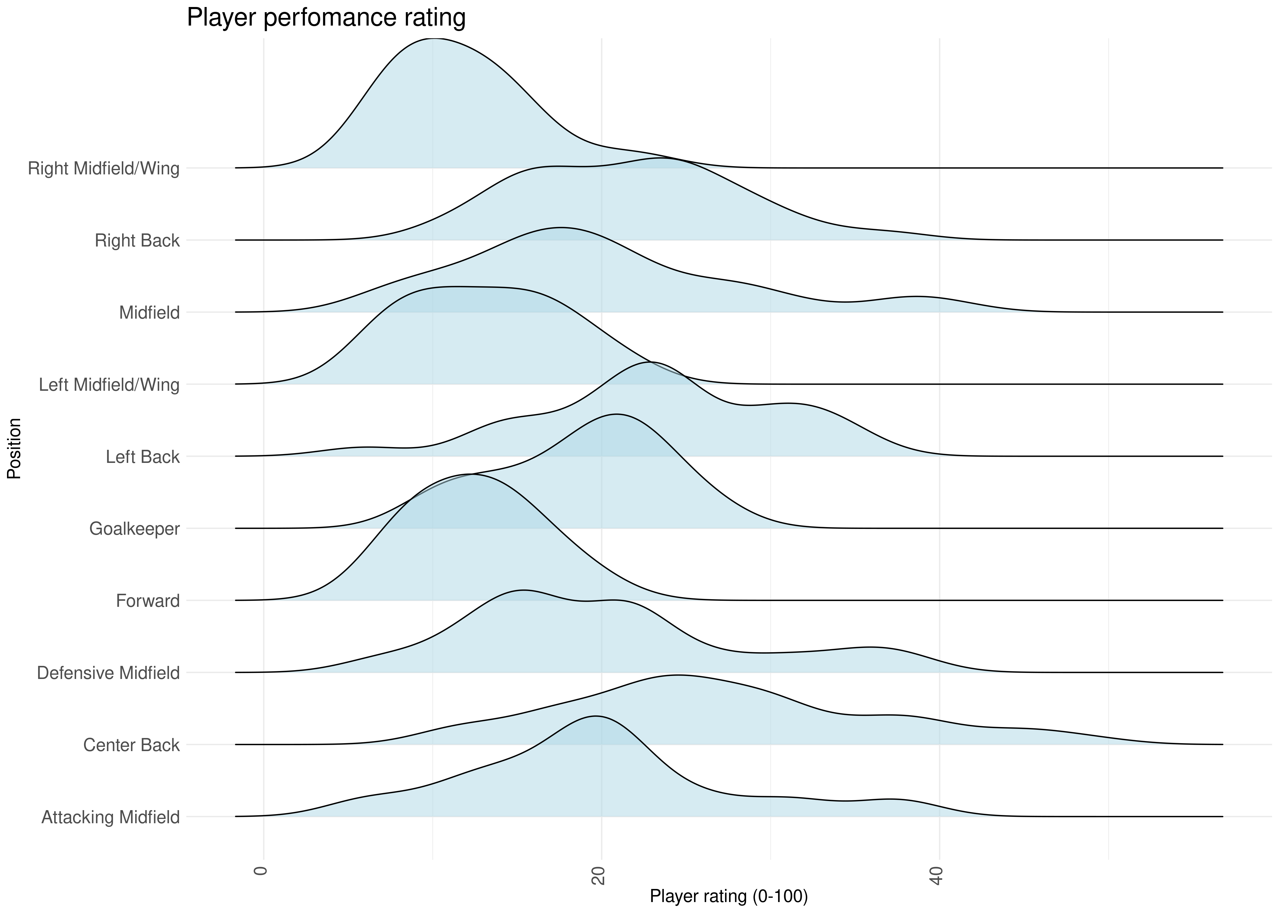
Let’s see the rating distribution for each position:
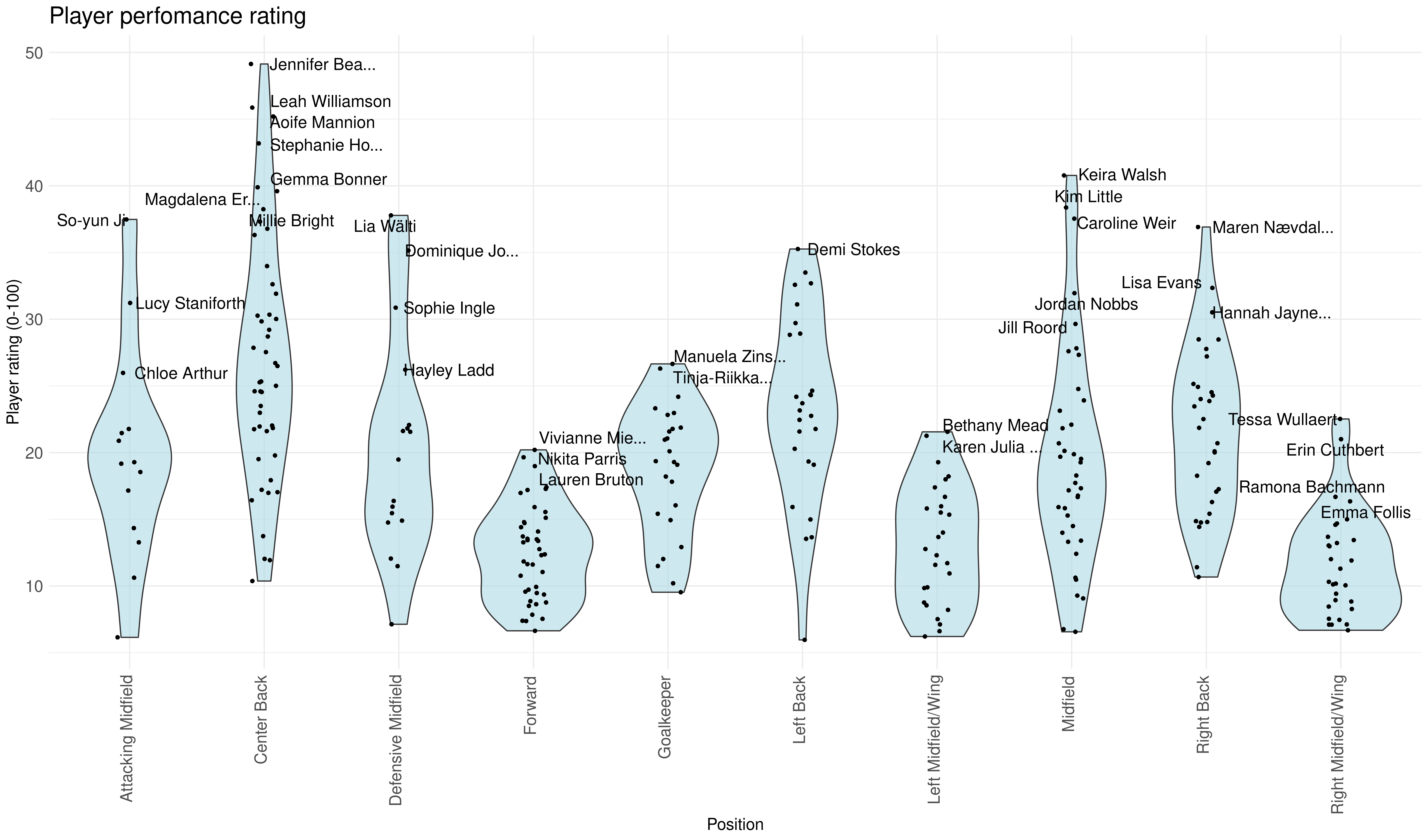
Let’s also take a look at the players with the highest rating. If anyone knows this league closely, let me know if these results seem reasonable!
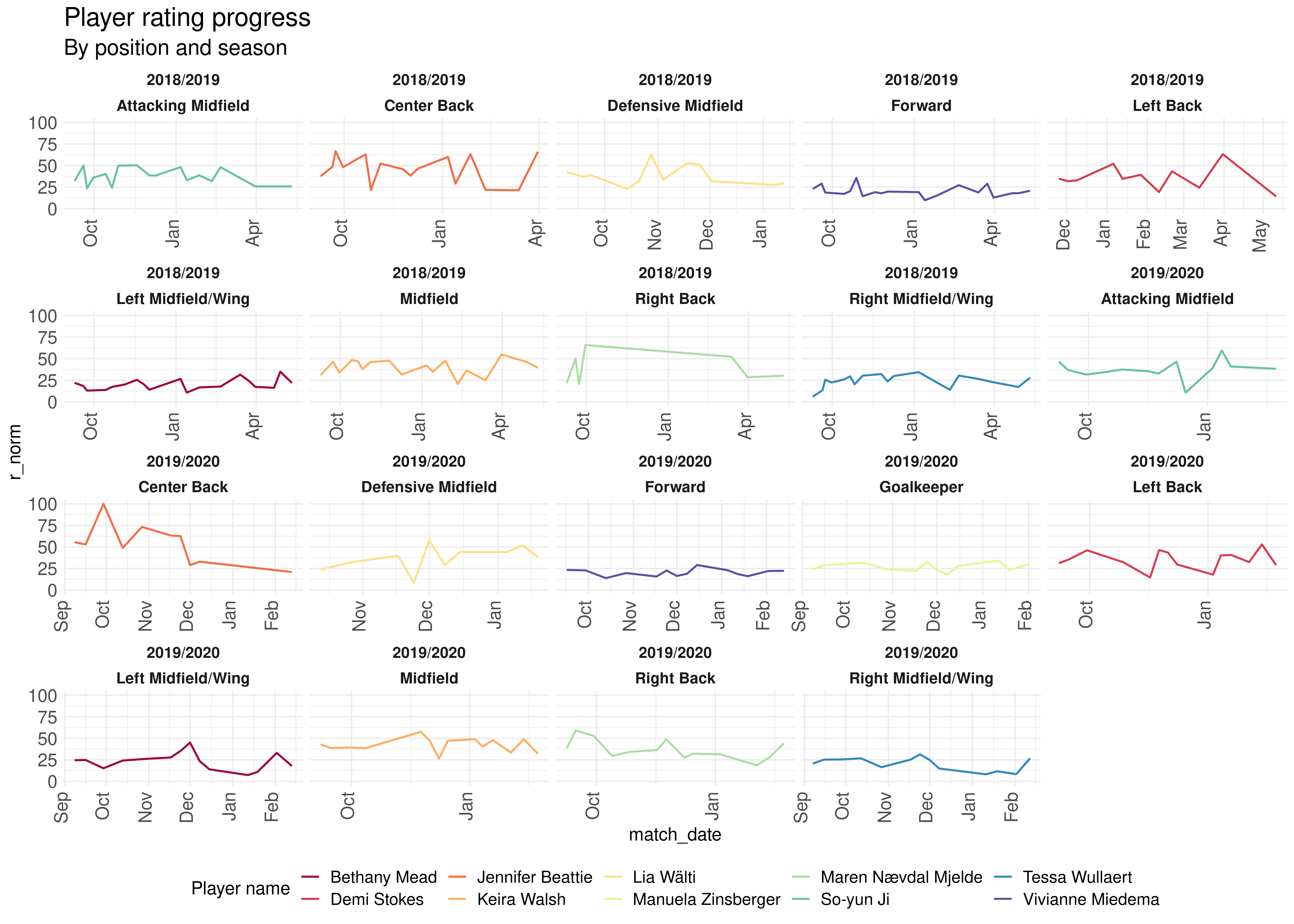
One last interesting thing we can see is the rating evolution over time.
Caveats and conclusions
This isn’t a perfect model and it doesn’t pretend to be either. Actually, what I find most interesting about the analysis is that with a relatively simple model you can get results that might be reasonable.
Some additional notes:
- Besides improving the model itself by including more variables or improving existing ones, I might consider training one model for each position instead of having only one.
- I’d be pretty skeptical of the goalkeepers’ results since their perfomance shouldn’t be measure in the same way as other players.
- Of course I’m not entirely comfortable with the way of building the \(r_i\) values. I’d probably look for a more sophisticated method.
- I’ve considered the players’ position as the way of comparing the performance within roles but this may not be the right way. PlayeRank goes one step further and compute the players’ roles via an affinity clustering.